Week 2

One week was over, I was well introduced to almost everyone in the office and now it was everything didn’t seem to be that strange to me.

I started to work with Excel and SQL fluently and i was completing the data analysis assignments that were given to me.

Day 1

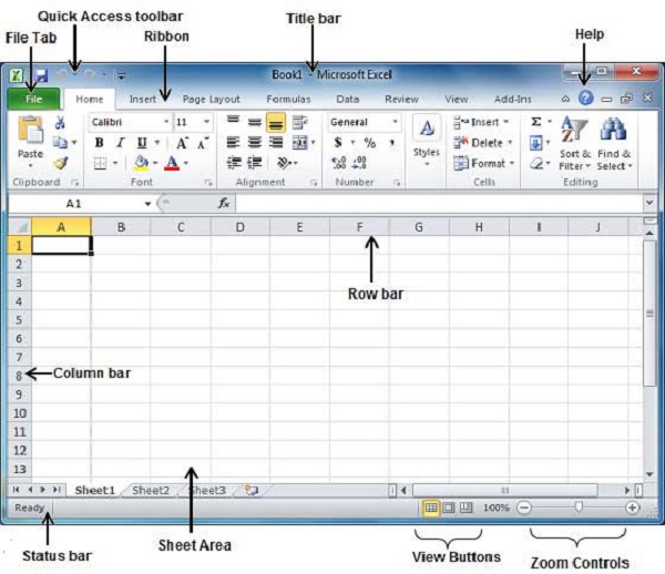
The following basic window appears when you start the excel application. Let us now understand the various important parts of this window.

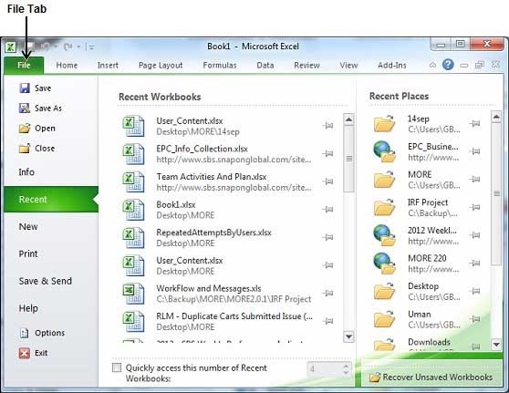
File Tab

The File tab replaces the Office button from Excel 2007. You can click it to check the Backstage view, where you come when you need to open or save files, create new sheets, print a sheet, and do other file-related operations.

Quick Access Toolbar

You will find this toolbar just above the File tab and its purpose is to provide a convenient resting place for the Excel’s most frequently used commands. You can customize this toolbar based on your comfort.

Ribbon

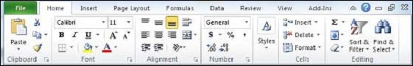
Ribbon contains commands organized in three components −

• Tabs − They appear across the top of the Ribbon and contain groups of related commands. Home, Insert, Page Layout are the examples of ribbon tabs.
• Groups − They organize related commands; each group name appears below the group on the Ribbon. For example, group of commands related to fonts or group of commands related to alignment etc.
• Commands − Commands appear within each group as mentioned above.

Title Bar

This lies in the middle and at the top of the window. Title bar shows the program and the sheet titles.

Help

The Help Icon can be used to get excel related help anytime you like. This provides nice tutorial on various subjects related to excel.

Zoom Control

Zoom control lets you zoom in for a closer look at your text. The zoom control consists of a slider that you can slide left or right to zoom in or out. The + buttons can be clicked to increase or decrease the zoom factor.

View Buttons

The group of three buttons located to the left of the Zoom control, near the bottom of the screen, lets you switch among excel’s various sheet views.

• Normal Layout view − This displays the page in normal view.
• Page Layout view − This displays pages exactly as they will appear when printed. This gives a full screen look of the document.
• Page Break view − This shows a preview of where pages will break when printed.

Sheet Area

The area where you enter data. The flashing vertical bar is called the insertion point and it represents the location where text will appear when you type.

Row Bar

Rows are numbered from 1 onwards and keeps on increasing as you keep entering data. Maximum limit is 1,048,576 rows.

Column Bar

Columns are numbered from A onwards and keeps on increasing as you keep entering data. After Z, it will start the series of AA, AB and so on. Maximum limit is 16,384 columns.

Status Bar

This displays the sheet information as well as the insertion point location. From left to right, this bar can contain the total number of pages and words in the document, language etc.

You can configure the status bar by right-clicking anywhere on it and by selecting or deselecting options from the provided list.

Dialog Box Launcher

This appears as a very small arrow in the lower-right corner of many groups on the Ribbon. Clicking this button opens a dialog box or task pane that provides more options about the group.

The Backstage view has been introduced in Excel 2010 and acts as the central place for managing your sheets. The backstage view helps in creating new sheets, saving and opening sheets, printing and sharing sheets, and so on.

Getting to the Backstage View is easy. Just click the File tab located in the upper-left corner of the Excel Ribbon. If you already do not have any opened sheet then you will see a window listing down all the recently opened sheets as follows −

If you already have an opened sheet then it will display a window showing the details about the opened sheet as shown below. Backstage view shows three columns when you select most of the available options in the first column.

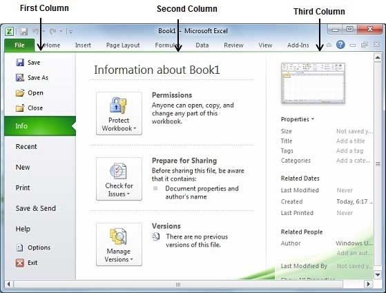
First column of the backstage view will have the following options −

S.No.	Option & Description
1	Save If an existing sheet is opened, it would be saved as is, otherwise it will display a dialogue box asking for the sheet name.
2	Save As A dialogue box will be displayed asking for sheet name and sheet type. By default, it will save in sheet 2010 format with extension .xlsx.
3	Open This option is used to open an existing excel sheet.
4	Close This option is used to close an opened sheet.
5	Info This option displays the information about the opened sheet.
6	Recent This option lists down all the recently opened sheets.
7	New This option is used to open a new sheet.
8	Print This option is used to print an opened sheet.
9	Save & Send This option saves an opened sheet and displays options to send the sheet using email etc.
10	Help You can use this option to get the required help about excel 2010.
11	Options Use this option to set various option related to excel 2010.
12	Exit Use this option to close the sheet and exit.

Sheet Information

When you click Info option available in the first column, it displays the following information in the second column of the backstage view −

• Compatibility Mode − If the sheet is not a native excel 2007/2010 sheet, a Convert button appears here, enabling you to easily update its format. Otherwise, this category does not appear.
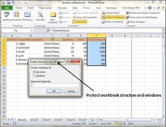
• Permissions − You can use this option to protect the excel sheet. You can set a password so that nobody can open your sheet, or you can lock the sheet so that nobody can edit your sheet.
• Prepare for Sharing − This section highlights important information you should know about your sheet before you send it to others, such as a record of the edits you made as you developed the sheet.
• Versions − If the sheet has been saved several times, you may be able to access previous versions of it from this section.

Sheet Properties

When you click Info option available in the first column, it displays various properties in the third column of the backstage view. These properties include sheet size, title, tags, categories etc.

You can also edit various properties. Just try to click on the property value and if property is editable, then it will display a text box where you can add your text like title, tags, comments, Author.

Exit Backstage View

It is simple to exit from the Backstage View. Either click on the File tab or press the Esc button on the keyboard to go back to excel working mode.

 

Day 2

Entering values in excel sheet is a child’s play and this chapter shows how to enter values in an excel sheet. A new sheet is displayed by default when you open an excel sheet as shown in the below screen shot.

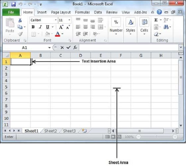
Sheet area is the place where you type your text. The flashing vertical bar is called the insertion point and it represents the location where text will appear when you type. When you click on a box then the box is highlighted. When you double click the box, the flashing vertical bar appears and you can start entering your data.

So, just keep your mouse cursor at the text insertion point and start typing whatever text you would like to type. We have typed only two words “Hello Excel” as shown below. The text appears to the left of the insertion point as you type.

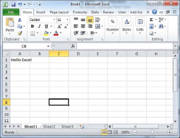
There are following three important points, which would help you while typing −

• Press Tab to go to next column.
• Press Enter to go to next row.
• Press Alt + Enter to enter a new line in the same column.

Entering values in excel sheet is a child’s play and this chapter shows how to enter values in an excel sheet. A new sheet is displayed by default when you open an excel sheet as shown in the below screen shot.

Sheet area is the place where you type your text. The flashing vertical bar is called the insertion point and it represents the location where text will appear when you type. When you click on a box then the box is highlighted. When you double click the box, the flashing vertical bar appears and you can start entering your data.

So, just keep your mouse cursor at the text insertion point and start typing whatever text you would like to type. We have typed only two words “Hello Excel” as shown below. The text appears to the left of the insertion point as you type.

There are following three important points, which would help you while typing −

• Press Tab to go to next column.
• Press Enter to go to next row.
• Press Alt + Enter to enter a new line in the same column.

 

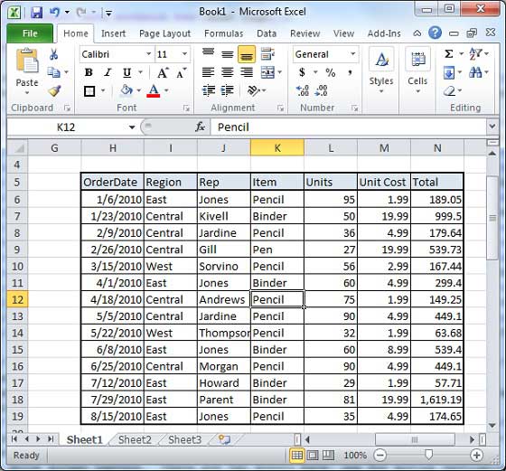
Excel provides a number of ways to move around a sheet using the mouse and the keyboard.

First of all, let us create some sample text before we proceed. Open a new excel sheet and type any data. We’ve shown a sample data in the screenshot.

OrderDate	Region	Rep	Item	Units	Unit Cost	Total
1/6/2010	East	Jones	Pencil	95	1.99	189.05
1/23/2010	Central	Kivell	Binder	50	19.99	999.5
2/9/2010	Central	Jardine	Pencil	36	4.99	179.64
2/26/2010	Central	Gill	Pen	27	19.99	539.73
3/15/2010	West	Sorvino	Pencil	56	2.99	167.44
4/1/2010	East	Jones	Binder	60	4.99	299.4
4/18/2010	Central	Andrews	Pencil	75	1.99	149.25
5/5/2010	Central	Jardine	Pencil	90	4.99	449.1
5/22/2010	West	Thompson	Pencil	32	1.99	63.68
6/8/2010	East	Jones	Binder	60	8.99	539.4
6/25/2010	Central	Morgan	Pencil	90	4.99	449.1
7/12/2010	East	Howard	Binder	29	1.99	57.71
7/29/2010	East	Parent	Binder	81	19.99	1,619.19
8/15/2010	East	Jones	Pencil	35	4.99	174.65

Moving with Mouse

You can easily move the insertion point by clicking in your text anywhere on the screen. Sometime if the sheet is big then you cannot see a place where you want to move. In such situations, you would have to use the scroll bars, as shown in the following screen shot −

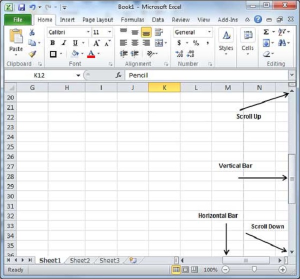
You can scroll your sheet by rolling your mouse wheel, which is equivalent to clicking the up-arrow or down-arrow buttons in the scroll bar.

Moving with Scroll Bars

As shown in the above screen capture, there are two scroll bars: one for moving vertically within the sheet, and one for moving horizontally. Using the vertical scroll bar, you may −

• Move upward by one line by clicking the upward-pointing scroll arrow.
• Move downward by one line by clicking the downward-pointing scroll arrow.
• Move one next page, using next page button (footnote).
• Move one previous page, using previous page button (footnote).
• Use Browse Object button to move through the sheet, going from one chosen object to the next.

Moving with Keyboard

The following keyboard commands, used for moving around your sheet, also move the insertion point −

Keystroke	Where the Insertion Point Moves
	Forward one box
	Back one box
	Up one box
	Down one box
PageUp	To the previous screen
PageDown	To the next screen
Home	To the beginning of the current screen
End	To the end of the current screen

You can move box by box or sheet by sheet. Now click in any box containing data in the sheet. You would have to hold down the Ctrl key while pressing an arrow key, which moves the insertion point as described here −

Key Combination	Where the Insertion Point Moves
Ctrl +	To the last box containing data of the current row.
Ctrl +	To the first box containing data of the current row.
Ctrl +	To the first box containing data of the current column.
Ctrl +	To the last box containing data of the current column.
Ctrl + PageUp	To the sheet in the left of the current sheet.
Ctrl + PageDown	To the sheet in the right of the current sheet.
Ctrl + Home	To the beginning of the sheet.
Ctrl + End	To the end of the sheet.

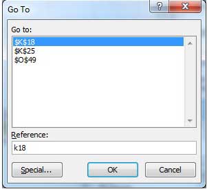
Moving with Go To Command

Press F5 key to use Go To command, which will display a dialogue box where you will find various options to reach to a particular box.

Normally, we use row and column number, for example K5 and finally press Go To button.

Day 3

Saving New Sheet

Once you are done with typing in your new excel sheet, it is time to save your sheet/workbook to avoid losing work you have done on an Excel sheet. Following are the steps to save an edited excel sheet −

Step 1 − Click the File tab and select Save As option.

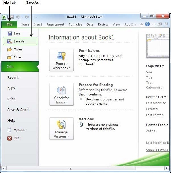
Step 2 − Select a folder where you would like to save the sheet, Enter file name, which you want to give to your sheet and Select a Save as type, by default it is .docx format.

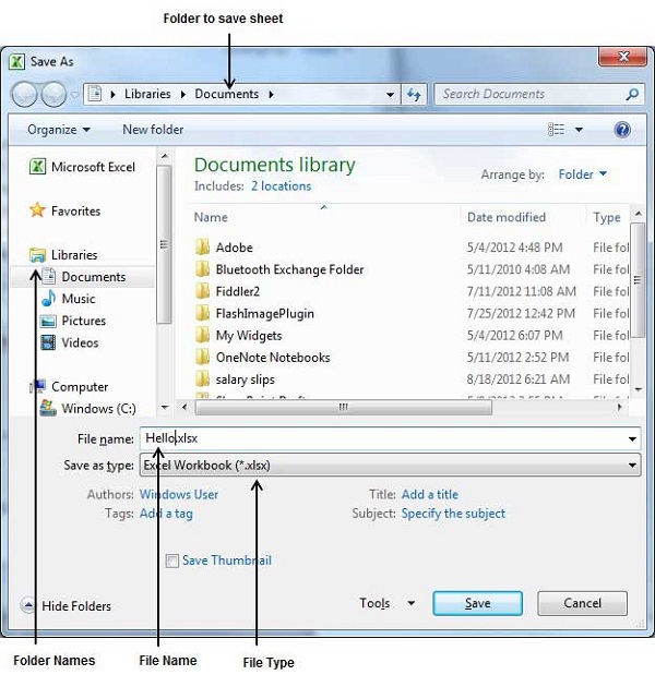
Step 3 − Finally, click on Save button and your sheet will be saved with the entered name in the selected folder.

Saving New Changes

There may be a situation when you open an existing sheet and edit it partially or completely, or even you would like to save the changes in between editing of the sheet. If you want to save this sheet with the same name, then you can use either of the following simple options −

• Just press Ctrl + S keys to save the changes.
• Optionally, you can click on the floppy icon available at the top left corner and just above the File tab. This option will also save the changes.
• You can also use third method to save the changes, which is the Saveoption available just above the Save As option as shown in the above screen capture.

If your sheet is new and it was never saved so far, then with either of the three options, word would display you a dialogue box to let you select a folder, and enter sheet name as explained in case of saving new sheet.

Saving New Sheet

Once you are done with typing in your new excel sheet, it is time to save your sheet/workbook to avoid losing work you have done on an Excel sheet. Following are the steps to save an edited excel sheet −

Step 1 − Click the File tab and select Save As option.

Step 2 − Select a folder where you would like to save the sheet, Enter file name, which you want to give to your sheet and Select a Save as type, by default it is .docx format.

Step 3 − Finally, click on Save button and your sheet will be saved with the entered name in the selected folder.

Saving New Changes

There may be a situation when you open an existing sheet and edit it partially or completely, or even you would like to save the changes in between editing of the sheet. If you want to save this sheet with the same name, then you can use either of the following simple options −

• Just press Ctrl + S keys to save the changes.
• Optionally, you can click on the floppy icon available at the top left corner and just above the File tab. This option will also save the changes.
• You can also use third method to save the changes, which is the Saveoption available just above the Save As option as shown in the above screen capture.

If your sheet is new and it was never saved so far, then with either of the three options, word would display you a dialogue box to let you select a folder, and enter sheet name as explained in case of saving new sheet.

Copy Worksheet

First of all, let us create some sample text before we proceed. Open a new excel sheet and type any data. We’ve shown a sample data in the screenshot.

OrderDate	Region	Rep	Item	Units	Unit Cost	Total
1/6/2010	East	Jones	Pencil	95	1.99	189.05
1/23/2010	Central	Kivell	Binder	50	19.99	999.5
2/9/2010	Central	Jardine	Pencil	36	4.99	179.64
2/26/2010	Central	Gill	Pen	27	19.99	539.73
3/15/2010	West	Sorvino	Pencil	56	2.99	167.44
4/1/2010	East	Jones	Binder	60	4.99	299.4
4/18/2010	Central	Andrews	Pencil	75	1.99	149.25
5/5/2010	Central	Jardine	Pencil	90	4.99	449.1
5/22/2010	West	Thompson	Pencil	32	1.99	63.68
6/8/2010	East	Jones	Binder	60	8.99	539.4
6/25/2010	Central	Morgan	Pencil	90	4.99	449.1
7/12/2010	East	Howard	Binder	29	1.99	57.71
7/29/2010	East	Parent	Binder	81	19.99	1,619.19
8/15/2010	East	Jones	Pencil	35	4.99	174.65

Here are the steps to copy an entire worksheet.

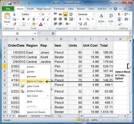
Step 1 − Right Click the Sheet Name and select the Move or Copy option.

Step 2 − Now you’ll see the Move or Copy dialog with select Worksheetoption as selected from the general tab. Click the Ok button.

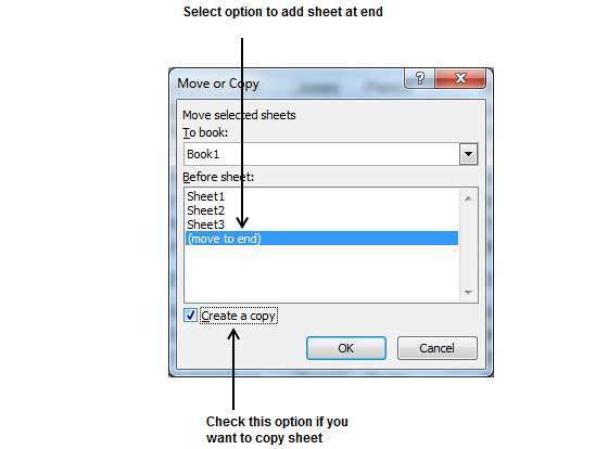
Select Create a Copy Checkbox to create a copy of the current sheet and Before sheet option as (move to end) so that new sheet gets created at the end.

Press the Ok Button.

Now you should have your copied sheet as shown below.

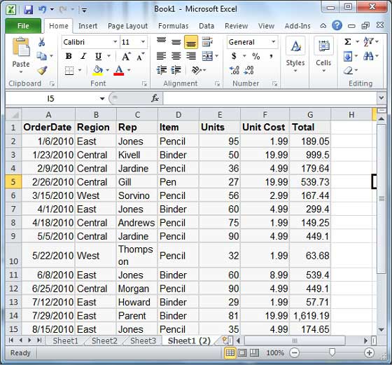
You can rename the sheet by double clicking on it. On double click, the sheet name becomes editable. Enter any name say Sheet5 and press Tab or Enter Key.

Day 3

Formatting Cell

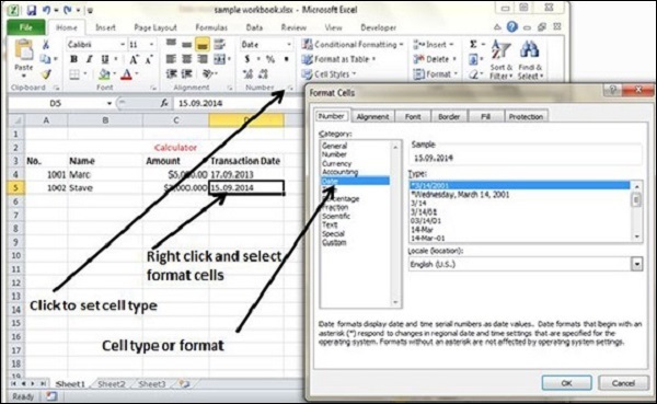
MS Excel Cell can hold different types of data like Numbers, Currency, Dates, etc. You can set the cell type in various ways as shown below −

• Right Click on the cell » Format cells » Number.
• Click on the Ribbon from the ribbon.

Various Cell Formats

Below are the various cell formats.

• General − This is the default cell format of Cell.
• Number − This displays cell as number with separator.
• Currency − This displays cell as currency i.e. with currency sign.
• Accounting − Similar to Currency, used for accounting purpose.
• Date − Various date formats are available under this like 17-09-2013, 17^th-Sep-2013, etc.
• Time − Various Time formats are available under this, like 1.30PM, 13.30, etc.
• Percentage − This displays cell as percentage with decimal places like 50.00%.
• Fraction − This displays cell as fraction like 1/4, 1/2 etc.
• Scientific − This displays cell as exponential like 5.6E+01.
• Text − This displays cell as normal text.
• Special − Special formats of cell like Zip code, Phone Number.
• Custom − You can use custom format by using this.

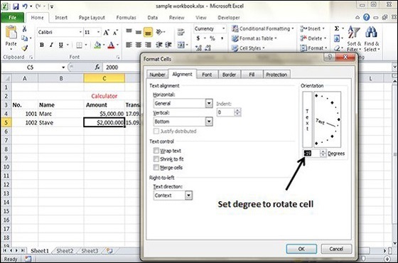
  You can rotate the cell by any degree to change the orientation of the cell.

  Rotating Cell from Home Tab

  Click on the orientation in the Home tab. Choose options available like Angle CounterClockwise, Angle Clockwise, etc.

  

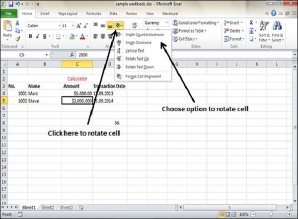
  Rotating Cell from Formatting Cell

  Right Click on the cell. Choose Format cells » Alignment » Set the degree for rotation.

  Merge Cells

  MS Excel enables you to merge two or more cells. When you merge cells, you don’t combine the contents of the cells. Rather, you combine a group of cells into a single cell that occupies the same space.

  You can merge cells by various ways as mentioned below.

  • Choose Merge & Center control on the Ribbon, which is simpler. To merge cells, select the cells that you want to merge and then click the Merge & Center button.

  

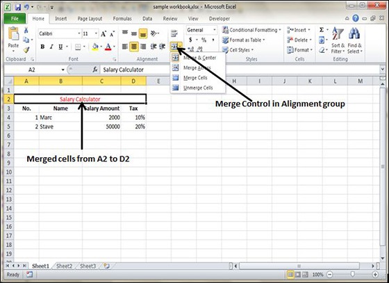
  • Choose Alignment tab of the Format Cells dialogue box to merge the cells.

  

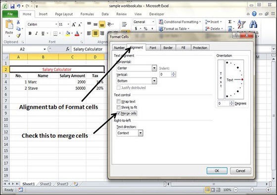
  Additional Options

  The Home » Alignment group » Merge & Center control contains a drop-down list with these additional options −

  • Merge Across − When a multi-row range is selected, this command creates multiple merged cells — one for each row.
  • Merge Cells − Merges the selected cells without applying the Center attribute.
  • Unmerge Cells − Unmerges the selected cells.

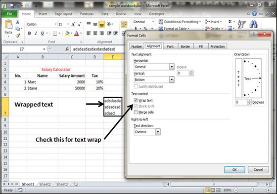
  Wrap Text and Shrink to Fit

  If the text is too wide to fit the column width but don’t want that text to spill over into adjacent cells, you can use either the Wrap Text option or the Shrink to Fit option to accommodate that text.

  

Day 4

Filters in MS Excel

Filtering data in MS Excel refers to displaying only the rows that meet certain conditions. (The other rows gets hidden.)

Using the store data, if you are interested in seeing data where Shoe Size is 36, then you can set filter to do this. Follow the below mentioned steps to do this.

• Place a cursor on the Header Row.
• Choose Data Tab » Filter to set filter.

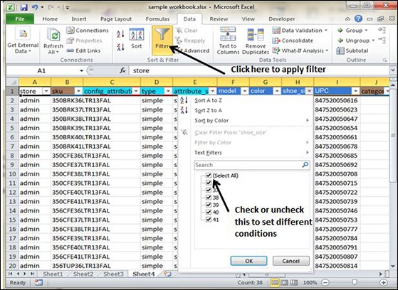
• Click the drop-down arrow in the Area Row Header and remove the check mark from Select All, which unselects everything.
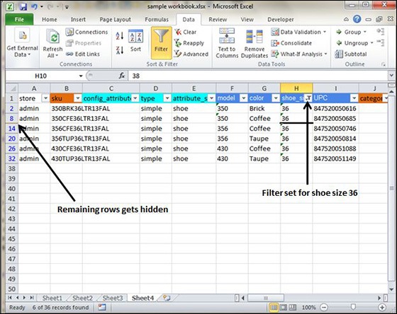
• Then select the check mark for Size 36 which will filter the data and displays data of Shoe Size 36.
• Some of the row numbers are missing; these rows contain the filtered (hidden) data.
• There is drop-down arrow in the Area column now shows a different graphic — an icon that indicates the column is filtered.

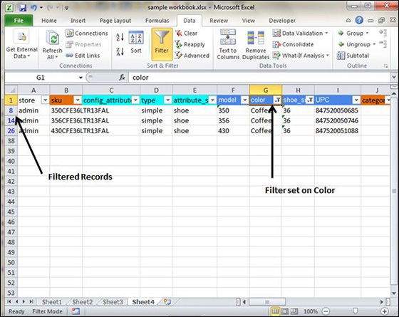
Using Multiple Filters

You can filter the records by multiple conditions i.e. by multiple column values. Suppose after size 36 is filtered, you need to have the filter where color is equal to Coffee. After setting filter for Shoe Size, choose Color column and then set filter for color.

Sorting in MS Excel

Sorting data in MS Excel rearranges the rows based on the contents of a particular column. You may want to sort a table to put names in alphabetical order. Or, maybe you want to sort data by Amount from smallest to largest or largest to smallest.

To Sort the data follow the steps mentioned below.

• Select the Column by which you want to sort data.
• Choose Data Tab » Sort Below dialog appears.

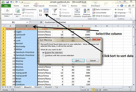
• If you want to sort data based on a selected column, Choose Continue with the selection or if you want sorting based on other columns, choose Expand Selection.
• You can Sort based on the below Conditions.
  • Values − Alphabetically or numerically.
  • Cell Color − Based on Color of Cell.
  • Font Color − Based on Font color.
  • Cell Icon − Based on Cell Icon.

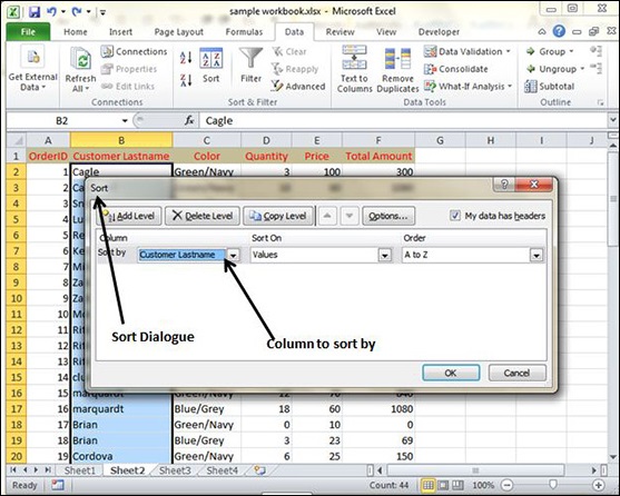
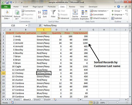
• Clicking Ok will sort the data.

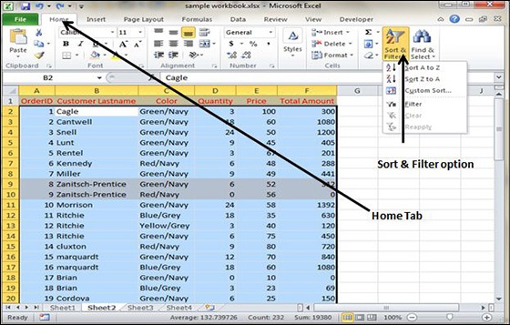
Sorting option is also available from the Home Tab. Choose Home Tab » Sort & Filter. You can see the same dialog to sort records.

Day 5

Data Tables

In Excel, a Data Table is a way to see different results by altering an input cell in your formula. Data tables are available in Data Tab » What-If analysis dropdown » Data table in MS Excel.

Data Table with Example

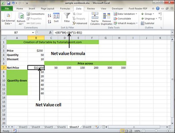
Now, let us see data table concept with an example. Suppose you have the Price and quantity of many values. Also, you have the discount for that as third variable for calculating the Net Price. You can keep the Net Price value in the organized table format with the help of the data table. Your Price runs horizontally to the right while quantity runs vertically down. We are using a formula to calculate the Net Price as Price multiplied by Quantity minus total discount (Quantity * Discount for each quantity).

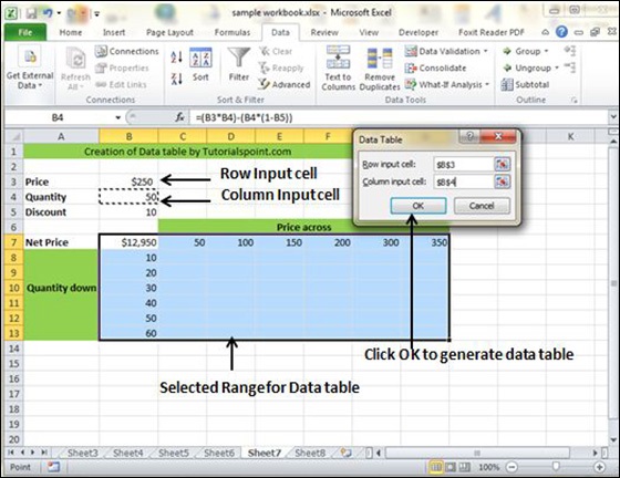
Now, for creation of data table select the range of data table. Choose Data Tab » What-If analysis dropdown » Data table. It will give you dialogue asking for Input row and Input Column. Give the Input row as Price cell (In this case cell B3) and Input column as quantity cell (In this case cell B4). Please see the below screen-shot.

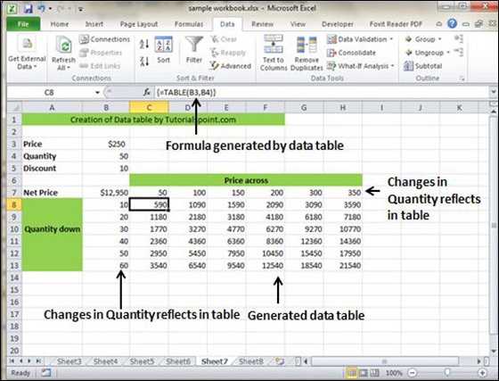
Clicking OK will generate data table as shown in the below screen-shot. It will generate the table formula. You can change the price horizontally or quantity vertically to see the change in the Net Price.

Pivot Tables

A pivot table is essentially a dynamic summary report generated from a database. The database can reside in a worksheet (in the form of a table) or in an external data file. A pivot table can help transform endless rows and columns of numbers into a meaningful presentation of the data. Pivot tables are very powerful tool for summarized analysis of the data.

Pivot tables are available under Insert tab » PivotTable dropdown » PivotTable.

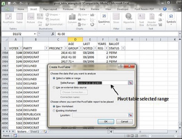
Pivot Table Example

Now, let us see Pivot table with the help of example. Suppose you have huge data of voters and you want to see the summarized data of voter Information per party, then you can use the Pivot table for it. Choose Insert tab » Pivot Table to insert pivot table. MS Excel selects the data of the table. You can select the pivot table location as existing sheet or new sheet.

This will generate the Pivot table pane as shown below. You have various options available in the Pivot table pane. You can select fields for the generated pivot table.

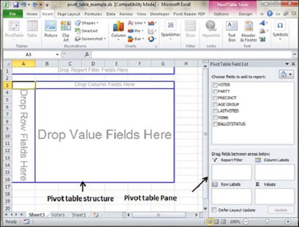
• Column labels − A field that has a column orientation in the pivot table. Each item in the field occupies a column.
• Report Filter − You can set the filter for the report as year, then data gets filtered as per the year.
• Row labels − A field that has a row orientation in the pivot table. Each item in the field occupies a row.
• Values area − The cells in a pivot table that contain the summary data. Excel offers several ways to summarize the data (sum, average, count, and so on).

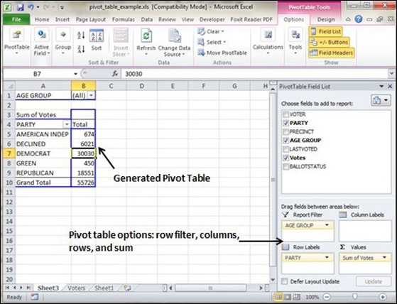
After giving input fields to the pivot table, it generates the pivot table with the data as shown below.

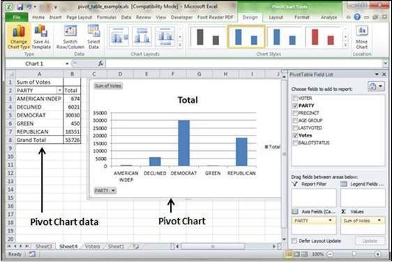
Pivot Charts

A pivot chart is a graphical representation of a data summary, displayed in a pivot table. A pivot chart is always based on a pivot table. Although Excel lets you create a pivot table and a pivot chart at the same time, you can’t create a pivot chart without a pivot table. All Excel charting features are available in a pivot chart.

Pivot charts are available under Insert tab » PivotTable dropdown » PivotChart.

Pivot Chart Example

Now, let us see Pivot table with the help of an example. Suppose you have huge data of voters and you want to see the summarized view of the data of voter Information per party in the form of charts, then you can use the Pivot chart for it. Choose Insert tab » Pivot Chart to insert the pivot table.

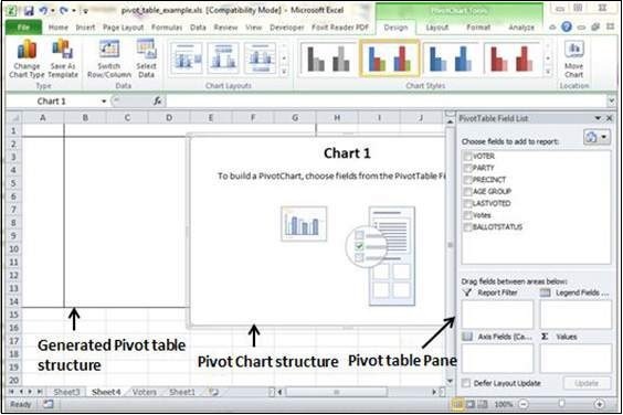
MS Excel selects the data of the table. You can select the pivot chart location as an existing sheet or a new sheet. Pivot chart depends on automatically created pivot table by the MS Excel. You can generate the pivot chart in the below screen-shot.